python众多文件中提取轮毂高度处风速
背景分析
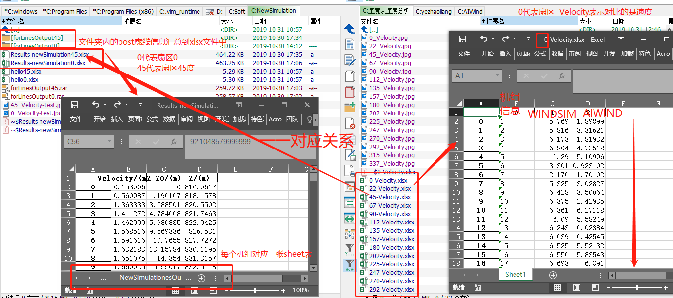
在前面的 python提取多个文件汇总到一个excel表一文中,我们使用ExcelWriter把提取的速度信息汇总在一个xls文件,各个sheet存放真实数据
而在AIWIND计算中,有可能插值错误,会出现Null值,于是a python提取多个文件的存在null速度廓线提出了过滤NULL值得方案
以上工作针对的是风廓线,我们现在想要从这个汇总表提取出来各个机位点在一定扇区下,比如0°得的轮毂高度处速度曲线, 也就是每计算一个扇区,我们都希望立马处理得到对应的对比结果,观察是否有所改进!于是做了下面工作
在python对比作图一文中加入了数据的导出功能,可在此基础上进行改写
下图中左边为瞬态扇区的AIWIND即时结果,右边为改进前的WINDSIM和AIWIND在各个扇区的对比图,我们希望AIWIND即时结果能够较好地吻合规律,与之前的WINDSIM结果做对比,即提取即时扇区下的各个机位点的速度廓线,汇总表格,遍历所有sheetnames,提取轮毂点位的速度信息,作图,也可以导出,当前未进行。
技术分解
- 依然利用脚本提取风廓线文件,一个扇区生成一个汇总表
- 遍历汇总表的所有sheetnames, 利用Excel_File()和parse的功能
- 利用列表数据结构+条件提取对应高度处的风速
技术实现
设计了一个plotSector,可针对对应扇区处理;
- 注意观察fileReadyAnalysis的及时结果存放位置?
- 注意观察对比作图导出的数据表格`0-Velocity.xlsx..`存放位置?
import os
import pandas as pd
import numpy as np
import matplotlib.pyplot as plt

## 注意需要有windsim各个扇区的数据 , 当前有一个问题必须配合AIIWND
#fileReadyAnalysis=r"C:\Users\yezhaoliang\Desktop\NewSimulation\Results-newSimulation45.xlsx"
#fileReadyAnalysis=r"C:\Users\yezhaoliang\Desktop\NewSimulation\Results-newSimulation0.xlsx"
## Sector: 0 22 45 67 90 112 135 157 180 202 247 270 292 315 337
plotSector='0'
## AIWIND导出的数据需要汇总
fileReadyAnalysis=r"C:\Users\yezhaoliang\Desktop\NewSimulation\Results-newSimulation"+plotSector+".xlsx"

if __name__ == "__main__":
    x_axix = ["T11", "T12", "T13", "T21", "T22", "T23", "T1", "T10", "T14", "T15", "T16", "T17", "T18", "T19", "T2", "T20",
              "T3", "T4", "T5", "T6", "T7", "T8", "T9", "366","387"];
    accordingTable = ["T1", "T2", "T3", "T4", "T5", "T6", "T7", "T8", "T9", "T10", "T11", "T12", "T13", "T14", "T15",
                      "T16", "T17", "T18", "T19", "T20", "T21", "T22", "T23", "366","387"];
    x_axisChange = ["1", "2", "3", "4", "5", "6", "7", "8", "9", "10", "11", "12", "13", "14", "15", "16", "17", "18",
                    "19", "20", "21", "22", "23" ];

    speedTableDir=r'C:\Users\yezhaoliang\Desktop\work\AIWind\processWindSim\速度表速度分析'
    speedTable=speedTableDir+r'\\'+plotSector+'-velocity.xlsx'
    speedTableData=pd.read_excel(speedTable,usecols=[2])
    # b = pd.read_excel(fileReadyAnalysis,None)
    # sheetnames=b.keys()
    # sheetvalues=b.values()
    #hubVelocities=np.zeros(sheetvalues.__len__())

    xlsx =pd.ExcelFile(fileReadyAnalysis)
    turbines=pd.Series([0]*25)
    turbineVelocity=pd.Series([0]*25,dtype='float')
    count=0
    ## 读取通过程序汇总的各个扇区的数据(各个机位点存储在相应sheet表中
    for sheetname in xlsx.sheet_names:
        pdtemp=xlsx.parse(sheetname)
        #print(pdtemp.iloc[5:20,2])
        #linreg = LinearRegression()
        newCount=accordingTable.index(x_axix[count])
        ## 机位点名字
        print(sheetname[-7:-4])
        turbines[newCount]=sheetname[-7:-4]
        ## 数据提取
        text1=pdtemp.iloc[0:100,2]
        text2=pdtemp.iloc[0:100,1]
        iMax=[i for i in range(len(text1)) if text1[i]>90]

        neededIndex=iMax[0]
        neededIndexSmaller=iMax[0]-1
        smallZ=text1[neededIndexSmaller]
        smallV=text2[neededIndexSmaller]

        bigZ = text1[neededIndex]
        bigV = text2[neededIndex]
       # yi=[y for y in pdtemp.iloc[0:100,1]]
       # linreg.fit(pdtemp.iloc[5:20,2], pdtemp.iloc[5:20,1])
        hub_height=90
        velocityPredict=(bigV-smallV)/(bigZ-smallZ)*(hub_height-smallZ)+smallV
#        velocityPredict= linreg.predict(hub_height)
        print(velocityPredict)
        turbineVelocity[newCount]=velocityPredict
        count=count+1
    df=pd.concat([turbines,turbineVelocity],axis=1)
    #df.to_excel('hello45.xlsx')
    df.to_excel(r'C:\Users\yezhaoliang\Desktop\NewSimulation\hello'+plotSector+'.xlsx')
    # speeTableSeries=pd.Series(speedTableData.values())
    # tempArray=pd.concat(turbineVelocity[0:23],speeTableSeries)
    #temp1=[x for x in speedTableData]
    #temp2=[y for y in turbineVelocity]
    #tempArray=[temp1,temp2]
    aiwindYaxis=turbineVelocity[0:23]
    windsimYaxis=speedTableData[0:23]
    #ylimMax=max(tempArray[1])
    #ylimMin=min(tempArray[1])

    ylimMax=8
    ylimMin=2
    # 开始画图

    plt.figure(figsize = (15,8))
    plt.title('Sector-'+plotSector+' Analysis',fontsize=32 )
    #plt.plot(x_axix, aiwindYaxis, marker='o', color='black', label='AIWIND')
    plt.plot(x_axisChange, aiwindYaxis, marker='o',markersize='9', color='red',markerfacecolor='grey',markeredgecolor='black',linestyle='solid', label='AIWIND',linewidth=3)
    #plt.plot(sub_axix, test_acys,marker='*', color='red', label='testing accuracy')
    #plt.plot(x_axix, windsimYaxis,marker='*', color='blue', label='WindSiM')
    plt.plot(x_axisChange, windsimYaxis,marker='*',markersize='9', color='black',markerfacecolor='grey',markeredgecolor='black',label='WindSiM',linewidth=3)
    #plt.plot(x_axix, thresholds, color='blue', label='threshold')
    plt.legend()  # 显示图例
    plt.margins(0)
    plt.grid()
    plt.ylim(ylimMin-1,ylimMax+1)
    plt.xlabel('Turbine Names',fontsize=24 )
    plt.ylabel('Velocity',fontsize=24 )
    plt.tick_params(axis='both',which='major',labelsize=24)
    plt.savefig(r"C:\Users\yezhaoliang\Desktop\NewSimulation\\"+plotSector+"_"+'Velocity-test'+".jpg",dpi = 900)
    #plt.show()
Related
叶昭良
Engineer of offshore wind turbine technique research
My research interests include distributed energy, wind turbine power generation technique , Computational fluid dynamic and programmable matter.